Mastering Reinforcement Learning Without Temporal Difference: A Divide and Conquer Approach

Introduction

Reinforcement learning (RL) traditionally relies on temporal difference (TD) learning to estimate value functions, but TD struggles with long-horizon tasks due to error accumulation. This guide presents an alternative paradigm: divide and conquer. Unlike TD-based methods, this approach scales well to complex, off-policy scenarios. Here, you'll learn how to implement RL without TD, using Monte Carlo returns and careful decomposition. By the end, you'll have a robust strategy for tackling challenging RL problems.

Mastering Reinforcement Learning Without Temporal Difference: A Divide and Conquer Approach — Source: bair.berkeley.edu

What You Need

Basic RL knowledge: Understand of on-policy vs off-policy RL, value functions, and Bellman equations.
Programming environment: Python with RL libraries (e.g., Gymnasium, Stable-Baselines3) or custom code.
Data source: Off-policy dataset (old experiences, human demos, or internet data) for training.
Compute resources: Moderate CPU/GPU for training and evaluation.

Step-by-Step Guide

Step 1: Recognize the Limitations of TD Learning

Temporal difference learning updates the Q-function using the Bellman equation:

Q(s, a) ← r + γ max_a' Q(s', a')

This bootstrapping causes errors in Q(s', a') to propagate backward. For long-horizon tasks, errors accumulate over many steps, making learning unstable. Off-policy RL exacerbates this because data may be outdated. To avoid TD, we must rely on Monte Carlo (MC) returns, which use actual rewards without bootstrapping. In step 2, we'll see how to combine MC with divide and conquer.

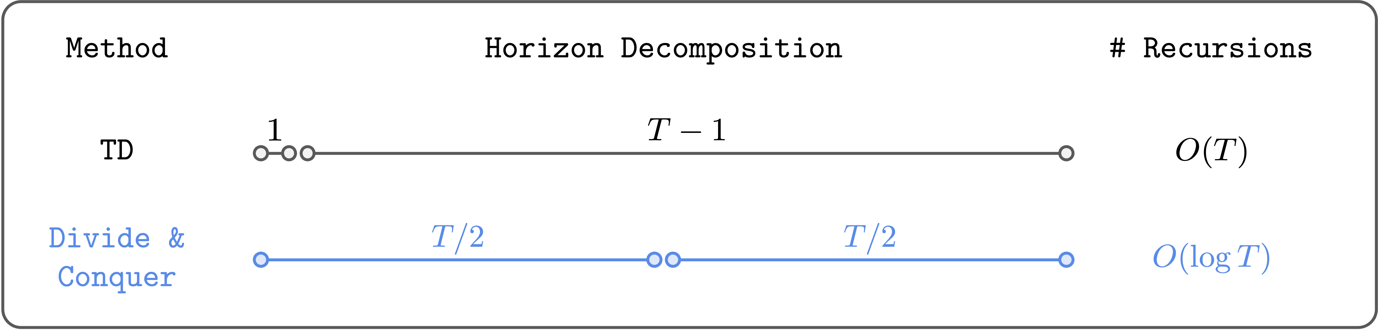
Step 2: Understand the Divide and Conquer Paradigm

The key insight: break the long horizon into smaller segments. Instead of learning from the entire trajectory, we use n-step returns. For a segment of length n, the target is:

G_t:t+n = r_t + γ r_t+1 + ... + γ^n-1 r_t+n-1 + γⁿ max_a' Q(s_t+n, a')

This hybrid reduces Bellman recursions by n times, limiting error propagation. As n grows, we approach pure MC (n = ∞). For off-policy data, you can use any n. Divide and conquer means you choose appropriate segment lengths based on task horizon.

Step 3: Set Up Your Off-Policy Environment

Off-policy RL allows using any data—old policies, demonstrations, or internet logs. Ensure your dataset contains trajectories with states, actions, rewards, and next states. No need for current policy rollout data. This is crucial when data collection is expensive (e.g., robotics). Prepare your data as a replay buffer. If using existing libraries, configure them for off-policy learning (e.g., DQN with replay memory).

Step 4: Implement Monte Carlo Returns Without Bootstrapping (Optional)

For pure MC learning (n = ∞), compute the full return from each state:

G_t = Σ_k=0^∞ γ^k r_t+k

Use the actual rewards from your dataset. Then set the Q-value target as G_t. No error propagation occurs. This works well for short episodes but may have high variance for long ones. That's why divide and conquer (step 2) is preferred: you can tune n for a bias-variance trade-off.

Step 5: Combine MC with Value Function Bootstrapping (n-step TD)

The recommended approach: use n-step returns where n is chosen to minimize error accumulation. Start with n = 10 or more, depending on task horizon. Update Q-values using the n-step target. This reduces the number of bootstrapping steps. Train your Q-network or tabular Q-table with these targets. Monitor the Q-value error: if it grows over time, increase n. If variance is too high, decrease n.

Step 6: Validate and Tune

Test your algorithm on a benchmark with long horizon (e.g., MuJoCo tasks with sparse rewards). Compare performance against standard TD methods (DQN, DDQN). You should see improved stability and faster convergence. Tune the hyperparameter n: start n = 10, then try 20, 50, 100. Also adjust learning rate and network architecture. Ensure you use off-policy data effectively—perform gradient updates on sampled batches.

Tips for Success

Start simple: Test with n-step TD before moving to pure MC. It's easier to debug.
Use importance sampling: If your data comes from a different policy, correct for distribution shift (though n-step MC already reduces bias).
Combine with model-based methods: For very long horizons, consider using learned models to generate synthetic rollouts.
Monitor error metrics: Track the Bellman error (TD error) or MC return variance to guide n selection.
Leverage existing implementations: Many libraries support n-step returns (e.g., Stable-Baselines3's DQN with n-step option).

By following these steps, you can implement a reinforcement learning algorithm that avoids the pitfalls of temporal difference learning. The divide and conquer approach scales gracefully to long-horizon tasks, making it ideal for real-world applications like robotics and healthcare.